Numerical Methods: 2010

jueves, 22 de julio de 2010

Jacobi Method

In numerical linear algebra, the Jacobi method is an algorithm for determining the solutions of a system of linear equations with largest absolute values in each row and column dominated by the diagonal element. Each diagonal element is solved for, and an approximate value plugged in. The process is then iterated until it converges. This algorithm is a stripped-down version of the Jacobi transformation method of matrix diagonalization. The method is named after German mathematician Carl Gustav Jakob Jacobi.

Given a square system of n linear equations:

$A\mathbf x = \mathbf b$

where:

$A=\begin{bmatrix} a_{11} & a_{12} & \cdots & a_{1n} \\ a_{21} & a_{22} & \cdots & a_{2n} \\ \vdots & \vdots & \ddots & \vdots \\a_{n1} & a_{n2} & \cdots & a_{nn} \end{bmatrix}, \qquad \mathbf{x} = \begin{bmatrix} x_{1} \\ x_2 \\ \vdots \\ x_n \end{bmatrix} , \qquad \mathbf{b} = \begin{bmatrix} b_{1} \\ b_2 \\ \vdots \\ b_n \end{bmatrix}.$

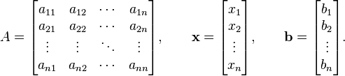
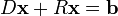
Then A can be decomposed into a diagonal component D, and the remainder R:

$A=D+R \qquad \text{where} \qquad D = \begin{bmatrix} a_{11} & 0 & \cdots & 0 \\ 0 & a_{22} & \cdots & 0 \\ \vdots & \vdots & \ddots & \vdots \\0 & 0 & \cdots & a_{nn} \end{bmatrix}, \qquad R = \begin{bmatrix} 0 & a_{12} & \cdots & a_{1n} \\ a_{21} & 0 & \cdots & a_{2n} \\ \vdots & \vdots & \ddots & \vdots \\a_{n1} & a_{n2} & \cdots & 0 \end{bmatrix}$

The system of linear equations may be rewritten as:

$(D + R )\mathbf{x} = \mathbf{b}$

$D \mathbf{x} + R \mathbf{x} = \mathbf{b}$

and finally:

$D \mathbf{x} = \mathbf{b} - R \mathbf{x}$

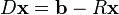
The Jacobi method is an iterative technique that solves the left hand side of this expression for x, using previous value for x on the right hand side. Analytically, this may be written as:

$\mathbf{x}^{(k+1)} = D^{-1} (\mathbf{b} - R \mathbf{x}^{(k)}).$

The element-based formula is thus:

$x^{(k+1)}_i = \frac{1}{a_{ii}} \left(b_i -\sum_{j\ne i}a_{ij}x^{(k)}_j\right),\quad i=1,2,\ldots,n.$

Note that the computation of x_i^(k+1) requires each element in x^(k) except itself. Unlike the Gauss–Seidel method, we can't overwrite x_i^(k) with x_i^(k+1), as that value will be needed by the rest of the computation. This is the most meaningful difference between the Jacobi and Gauss–Seidel methods, and is the reason why the former can be implemented as a parallel algorithm, unlike the latter. The minimum amount of storage is two vectors of size n.

Gauss Seidel Method

Gauss-Seidel Method

The Gauss-Seidel method (called Seidel's method by Jeffreys and Jeffreys 1988, p. 305) is a technique for solving the

equations of the linear system of equations

one at a time in sequence, and uses previously computed results as soon as they are available,

x_i^((k))=(b_i-sum_(j<i)a_(ij)x_j^((k))-sum_(j>i)a_(ij)x_j^((k-1)))/(a_(ii)).

There are two important characteristics of the Gauss-Seidel method should be noted. Firstly, the computations appear to be serial. Since each component of the new iterate depends upon all previously computed components, the updates cannot be done simultaneously as in the Jacobi method. Secondly, the new iterate

depends upon the order in which the equations are examined. If this ordering is changed, the components of the new iterates (and not just their order) will also change.

In terms of matrices, the definition of the Gauss-Seidel method can be expressed as

where the matrices

, and

represent the diagonal, strictly lower triangular, and strictly upper triangular parts of

, respectively.

The Gauss-Seidel method is applicable to strictly diagonally dominant, or symmetric positive definite matrices

martes, 20 de julio de 2010

MATRIX

SERIE TAYLOR

serie taylor

lunes, 28 de junio de 2010

Fixed Point Iteration

METODOS ABIERTOS

FALSE POSITON METHOD

False Position Method

miércoles, 26 de mayo de 2010

THE BISECTION METHOD

the bisection method. Given a nonlinear function f(x), we seek a value of x for which

f(x) = 0

Such a solution value for x is called a root of the equation, and a zero of the

function f(x).

The essence of the bisection method lies in the fact that the sign of a function f(x) changes on opposite sides of a root. Suppose the function f(x) has one root in the interval between x = a and x = c, or [a,c], as shown in the Figure below.

The bisection method is based on the fact that when an interval [a,c] contains a

root, the sign of the function at the two ends (f(a) and f(c)) are opposite each

other, namely

f(a)*f(c) < 0

The first step in the bisection method is to bisect the interval [a,c] into two

halves, namely [a,b] and [b,c], where

b=(a + b)/2

By checking the sign of

f(a)*f(b)

the half-interval containing the root can be identified. If

f(a)*f(b) < 0

then, the interval [a,b] has the root, otherwise the other interval [b,c] has the

root. Then the new interval containing the root is bisected again. As the procedure is repeated the interval becomes smaller and smaller. At each step, the midpoint of the interval containing the root is taken as the best approximation of the root. The iterative procedure is stopped when the halfinterval size is less than a prespecified size.

This method is illustrated in the following flowchart.

lunes, 24 de mayo de 2010

Roots of Equations

lunes, 17 de mayo de 2010

Darcy Law

Henry Darcy (1803 to 1858) invented the modern style Pitot tube, was the first researcher to suspect the existence of the boundary layer in fluid flow, contributed in the development of the Darcy-Weisbach equation for pipe flow resistance, made major contributions to open channel flow research and of course developed Darcy's Law for flow in porous media. His Law is a foundation stone for several fields of study including ground-water hydrology, soil physics, and petroleum engineering.

martes, 11 de mayo de 2010

CIPHER SIGNIFICANT

We can define the concept of significant cipher as that which provides unambiguous information about a specific experimental measurement.

All nonzero numbers expressing quantities equal to or greater than the experimental uncertainty are significant.
All zeros between significant digits are significant.
in a number with digits to the right of the decimal zeros to the right of last nonzero numbers are significant.

lunes, 10 de mayo de 2010

Mathematic Model

Mathematical models of reality are the vastly more important type of representation. Essentially, anything in the physical or biological world, whether natural or involving technology and human intervention, is subject to analysis by mathematical models if it can be described in terms of mathematical expressions. Thus, optimization and control theory may be used to model industrial processes, traffic patterns, sediment transport in streams, and other situations; information theory may be used to model message transmission, linguistic characteristics, and the like; and dimensional analysis and computer simulation may be used to model atmospheric circulation patterns, stress distribution in engineering structures, the growth and development of landforms, and a host of other processes in science and engineering.

lunes, 3 de mayo de 2010

Numerical Methods in Engineering

Numerical Analysis

Numerical Analysis is the study of algorithms that use numerical approximation for the problems of continuous mathematics .

Numerical analysis naturally finds applications in all fields of engineering and the physical sciences,
but in the 21^st century, the life sciences and even the arts have adopted elements of scientific computations. Ordinary differential equations appear in the movement of heavenly bodies; optimization occurs in portfolio management; numerical linear algebra is important for data analysis; stochastic differential equations and Markov chains are essential in simulating living cells for medicine and biology.
Before the advent of modern computers numerical methods often depended on hand interpolation in large printed tables. Since the mid 20th century, computers calculate the required functions instead.